In our publication
Learning state machines from data streams: A generic strategy and an improved heuristic
we introduced an algorithm learning probabilistic automata from data streams. Probabilistic
means that parsing the automaton with a string will yield its probability to occur, information
that is interesting when identifying rare events of the data stream. Rare events are intesting
in the domain of anomaly detection and can e.g. pose network threats on a network or rare
execution traces in software systems.
However, a problem of the algorithm is how to know how close its estimates actually are
to the real distribution. Statistics tells us that the more samples we gather
the more certain we can be about
our predictions. Therefore, the more samples a node in our automaton sees the more likely
its predicted probabilities will resemble the true probabilities, but we can never be certain.
This is a problem inherent to machine learning frameworks and has been studied by famous statisticians
such as Vladimir Vapnik and Alexey Chervonenkis, who are famous for their VC-dimension, a concept of
statistical learning theory.
Another approach to estimate the learning capacity of a statistical learner is a formal proof of
PAC-bounds (PAC=Probably Approximately Correct). We take this approach to show the correctness
of our algorithm in the extended version of our publication, found
here. However, because the proof is long and has lots of mathematical details I outline its main ideas
and steps in this blog post. For simplicity I use the same notation as in the paper, thus this blogpost
is a complemetary piece to the original proof. With that said, let's dive in with the definition of
PAC-bounds and why we use them.
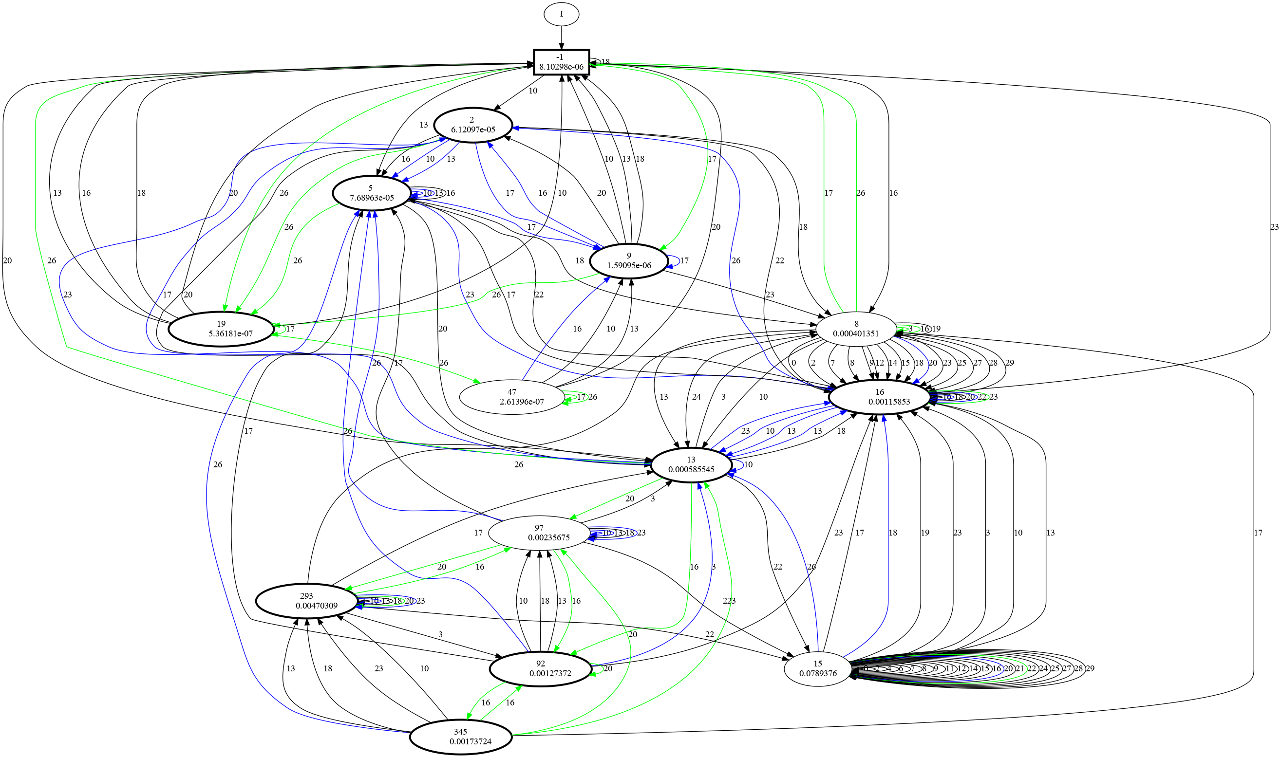
Example of a model we once learned. Traversing the graph yields probabilities of related events
happening, and we want to error bound these probabilities, making sure that the result is correct.
Definition of PAC-bounds
Why proving PAC-bounds? Usually when developing algorithms the developer will provide a proof
of correctness. This is a formal proof using mathematical methods showing that an algorithm
outputs the correct result for each input that it is designed for. In other words, a proof
of correctness shows that an algorithm works and gives correct output.However, many algorithms,
including many machine learning algorithms, rely on statistics, and there is no such thing as a
correct input and a corresponding correct output. Therefore, proofs of correctness are hard to
define for such algorithms.
PAC-bounds aim to close this gap. They are a statistical framework that provides statistical guarantees
on the goodness of the approximation quality a learning algorithm can achieve, given it sees enough samples.
More formally, the definition of PAC-bounds are as follows:
Definition: The Probably Approximately Correct (PAC) learning framework is
a framework to analyze machine learning algorithms. Formally, we are given a class of distributions
$\mathcal{D}$ over some set $X$, where $X$ remains fixed. A machine learning algorithm then PAC-learns
$\mathcal{D}$ if for each $\delta>0$ and each $\epsilon > 0$ the algorithm takes $S(\frac{1}{\epsilon},
\frac{1}{\delta}, |D|)$ i.i.d. drawn samples from a $D \in \mathcal{D}$ and returns a hypothesis $H$ s.t.
$L_1(D, H) \leq \epsilon$. In this notation, $|D|>0$ is a measure of complexity over $\mathcal{D}$. We
say a PAC learner is efficient if $S( \cdot )$ and $T( \cdot )$ are polynomial in all their respective
parameters.
$L_1$ in this definition is the $L_1$-distance, which is a measure for the
maximum sum of errors the output $H$ produces when compared with $D$. This definition essentially tells us
that if we have a PAC-learner, and we let it learn a problem, then the learner learns the target distribution
$D$ with a maximum sum of errors of $\epsilon$, for any chosen maximum error $\epsilon$, with a probability
$1-\delta$, if samples are provided i.i.d. from the target distribution. Pretty cool I'd say.
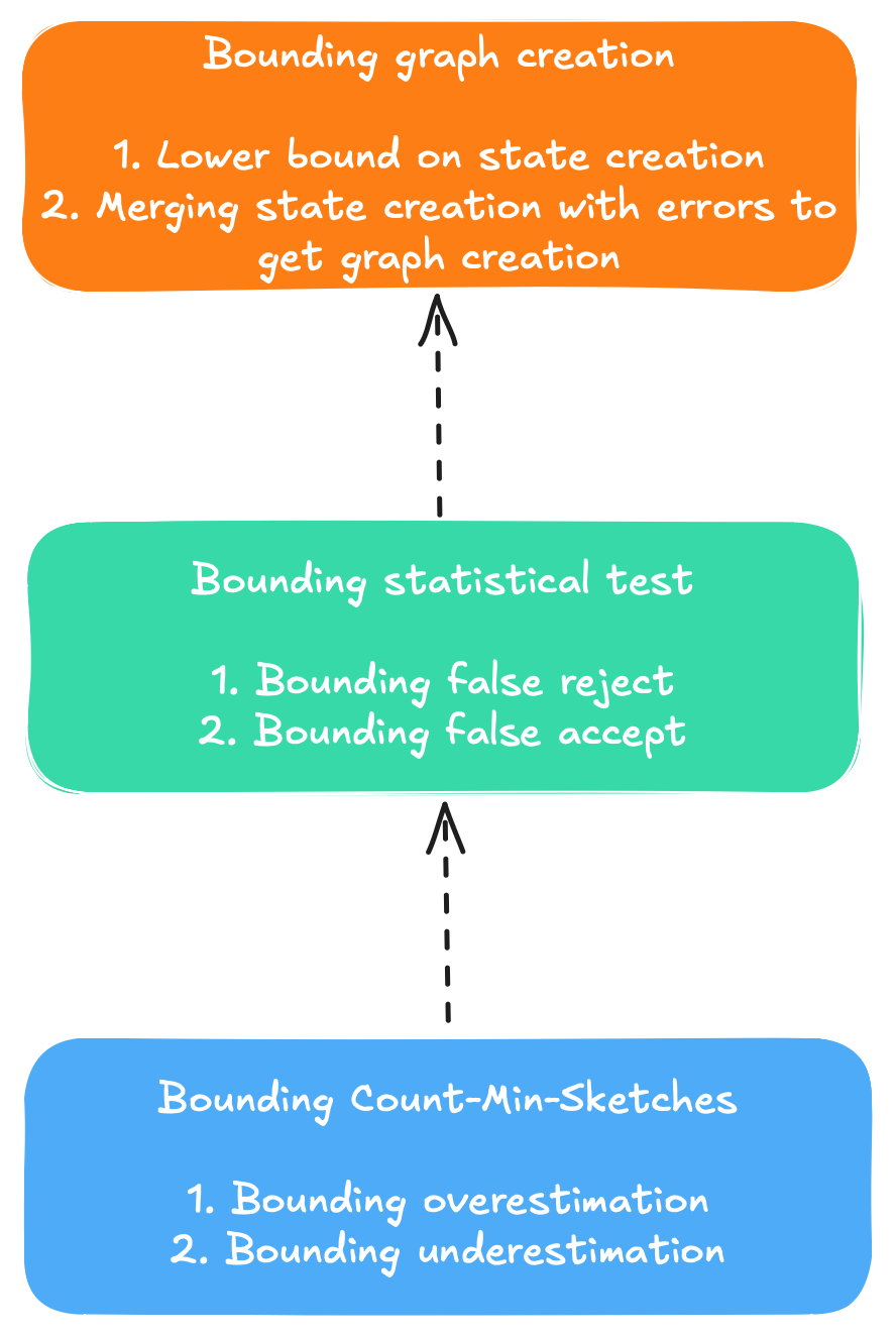
Steps for proof of PAC-bounds, from bottom to top.Steps for proof of PAC-bounds, from bottom to top.
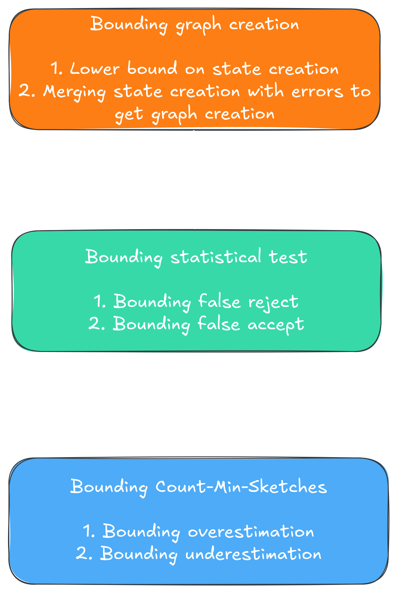
Bounds on Count-Min-Sketches
In order to show formal PAC-bounds we have to build them from the ground up, as shown in the figure above.
We have to start with the smallest unit of operation in our algorithm, show that we can probabilistically bound the error
they produce, and move it up layer by layer until we cover the whole algorithm. In our publication we chose Count-Min-Sketches
(CMS) as the most basic data structure. Hence, we first have to show that the CMS and the operations we perform on them are bounded.
We store samples distributions in the CMS and test with the Hoeffding-bound whether the two sampled distributions are
equal or not. If two sampled distributions, retrieved from the CMS and denoted with $\frac{\hat{c}_{\sigma_{q_i}}}{n_{q_i}}$, satisfy
$$\left| \frac{\hat{c}_{\sigma_{q_1}}}{n_{q_1}} - \frac{\hat{c}_{\sigma_{q_2}}}{n_{q_2}} \right| > \sqrt{\frac{1}{2}log
\left(\frac{2}{\alpha}\right)}\left(\frac{1}{\sqrt{n_{q_1}}}+\frac{1}{\sqrt{n_{q_2}}}\right),$$
then we consider them equal. The challenge we face now is that the CMS data structure works similar to a multiset. But unlike a
multiset it does not return exact counts, instead approximate counts. It is thus a memory saving data structure to count elements
of a data stream, where the cardinality of elements to store is either unknown before runtime, or simply too large. In short, the
sampled distributions we get from the CMS come with an error induced by estimating the sampled counts.
Since only the left hand side of the Hoeffding-bound depends on the statistics we draw, and the right hand side is only dependent
on the total size of samples it suffices to show that the left hand side is error bounded. If the error on the left hand side is
zero, the sampled frequencies are the real ones and the approximation effect of the CMS is zero. We can make two kinds of mistakes
here: We can overestimate or underestimate the true value on the left hand side of the equation. We start bounding the overestimation:
Theorem 1: Given the parameters ($\beta$, $\gamma$), and given two CMS whose width $w$ and depth $d$ of a CMS assume
$w=\left\lceil{\frac{e}{\beta}}\right\rceil$ and $d=\left\lceil{\ln \frac{1}{\gamma}}\right\rceil$. The error on the left hand
side of the Hoeffding-test is upper-bounded by $\beta$ with probability at least $1-2\gamma$.
In order to proof the theorem we start with the error bounds on the CMS given by the
original authors of the data structure,
and we define a new random variable from their approach using indicator variables. Subsequently we use the Markov bound
$$ P(X>a) \leq \frac{E(X)}{a} $$
to bound the random variable, showing that the divergence from the expectation value of the left hand side of the Hoeffding test above
is bounded. However, this proof only works when the left hand side's term before taking the absolute value is larger than or equal to
zero. Next we bound the case of underestimating the left hand side:
Theorem 2: With a probability of at least $1-2\gamma$ the left hand side of the Hoeffding-test with CMS is not underestimated by an offset
larger than $\beta$.
The proof is similar to the one of Theorem 1, so we can skip the explaination here. Last but not least we need to combine the two bounds.
The two cases can be generously bound using the union bound, a useful tool in general. From
$$P(A \cup B)= P(A) + B(B) - P(A \cap B) \leq P(A) + P(B)$$
we obtain the union bound as
$$ P(\cup_i A_i) \leq \sum_i P(A_i).$$
This settles our score with the CMS.
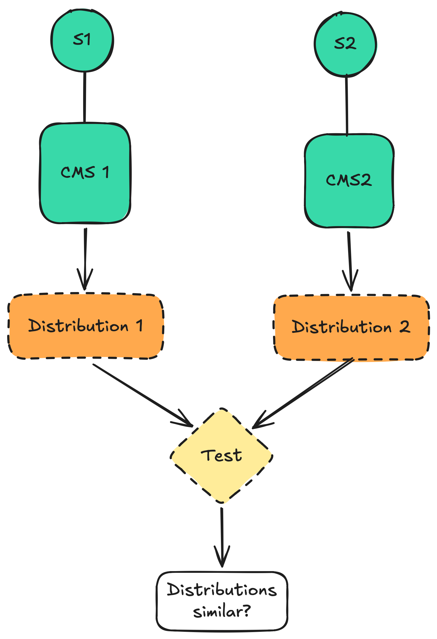
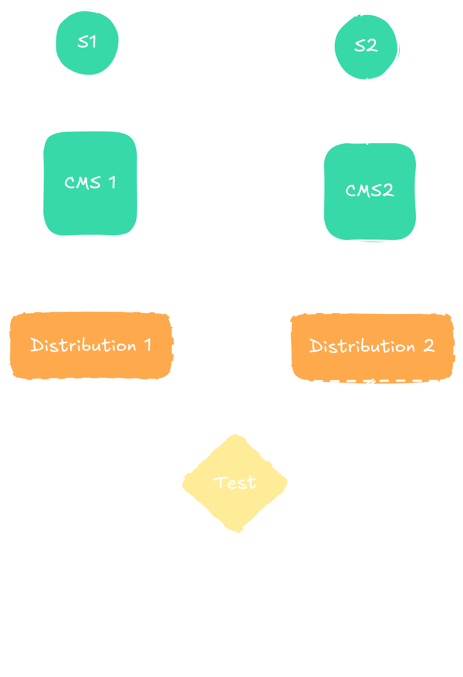
Comparing two states. Each state has one CMS, through which we can retrieve a sampled distribution
over input words. The two distributions are then compared through a statistical test. Mistakes can happen in the
statistical test and in retrieving the sampled distributions.
Comparing two states. Each state has one CMS, through which we can retrieve a sampled distribution
over input words. The two distributions are then compared through a statistical test. Mistakes can happen in the
statistical test and in retrieving the sampled distributions.
Bounds on statistical test
Having bound the error on the CMS data structure, knowing what can happen when we approximate the sampled distributions, rather than having the actual one,
we can move toward seeing what happens when we want to perform the actual statistical test on them. We will also have to reason about
how many samples to read in order to get good statistics in first place. We start with wondering about how many samples to read for a state to even get created.
The following theorem gives us no precise answer, but an intuition of how data samples from the data stream propagate through the tree representing the unmerged
automaton:
Theorem 3: Given batch-size $B$, upper bound on state $n$, and $p_{min}$ the minimum transition probability
$\lambda_{min}=\min_{i, j} \lambda(q_i, a_j)$. The algorithm reads $\mathcal{O}(nBN_{max})$ samples from the stream, where
$\mathbb{E}[|\lambda(q', a')|] = N_{max} \cdot \lambda_{min}$, with $q', a'$ chosen s.t. $\lambda_{min}=\lambda(q', a')$.
Here, $n$ is an upper bound on the states that are expected of the final automaton. Technically we do not need this hyperparameter
in a practical scenario, but we need it to show PAC-bounds. For more details on that see
this publication
by Palmer and Goldberg, which has greatly served as a guideline while constructing out own proof. What the theorem then tells us in simple terms is that
we know that there must a minimum non-zero transition probability within the automaton. Once we know that transition probability we can define an
expected constant proportional to the inverse of the minimum probability, and then the maximum number of expected samples grows linearly in
the number of states and the batch size. While not needed for the remainder, it is still nice to know that we can bound how many i.i.d. samples
the algorithm needs. The proof follows again via the Markov bound and proof by induction.
With that in mind we move on bounding the probability of
making a mistake in the statistical test. An error can either be a false reject (should merge those two states, but choose not to), or a false accept
(should not merge those two states, but actually choose to merge). We first look at the probability of a false reject when the CMS are correct:
Theorem 4: Given the Hoeffding-test as defined earlier, and assuming no collisions happened in the CMS, then the probability of a false reject
is kept below $2\alpha$.
We get this bound for free by using the same test as
Carrasco and Oncina.
The test is essentially a clever reformulation of the classical Hoeffding-bound, where they inject an $\alpha$
parameter that serves as an upper bound for the error. We can simply use their results here. However, the probability for
a false reject we'll have to bound on our own. We introduce a notion for what it means to distinguish two distributions:
Definition 1: We call two distributions $D_1$ and $D_2$ $\mu$-distinguishable when $L_{\infty}^p(D_1, D_2) \geq \mu$. We call a PDFA $T$ $\mu$-distinguishable when
$\forall q_1, q_2\in T: L_{\infty}^p\left(D_{q1}, D_{q2}\right) \geq \mu$.
This definition simply tells us that we use a threshold, and if the maximum distance is larger than it we say the distributions are not the same. We call this threshold
$\mu$, and we want it to be the maximum induced distance between two distributions. Now with that definition we can go to the following, more interesting theorem
about the bound for a false accept:
Theorem 5: Assuming the target PDFA we are trying to learn is $\mu$-distinguishable, there exists a minimum sample size $m_0$ per state such that the probability
of a false accept per state-pair is bounded by $\frac{\delta'}{2n^2|\Sigma|^2}$ under the assumption of no collisions.
Assuming that the target PDFA is $\mu$-distinguishable is a reasonable assumption and a simple mathemcatical formulation. The proof for this theorem follows by first
modeling the variance term using the indicator variables used earlier too, and then bounding it using Cauchy-Schwarz. Subsequently using the Chebychev-Cantelly inequality
for the lower tail
$$P(X - \mathbb{E}[X] \leq -\lambda) \leq \frac{Var(X)}{Var(X) + \lambda^2},$$
with $Var(X)$ being the variance we earlier bounded, we get the result using a clever substitute for $\lambda$.
After that we have to
move the CMS back into the picture. We already know that we can bound the error on the CMS, and we know what happens when they do not do any mistakes. The following theorems
describe what happens when they actually do make mistakes, starting with false accepts:
Theorem 6: Given the Hoeffding-test and given two frequencies estimated via CMS, allowing for collisions. Then the probability of a false accept under an updated Hoeffding-bound
$\sqrt{\frac{1}{2}log\left(\frac{2}{\alpha}\right)}\left(\frac{1}{\sqrt{m_1}}+\frac{1}{\sqrt{m_2}}\right) - \beta$ is bounded by $\frac{\delta_2'}{2n^2|\Sigma|^2}$.
And of course we also need to updated our analysis on false rejects.
Theorem 7: Narrowing the Hoeffding-test via $\sqrt{\frac{1}{2}log\left(\frac{2}{\alpha}\right)}\left(\frac{1}{\sqrt{m_1}}+\frac{1}{\sqrt{m_2}}\right) - \beta$, the upper bound for
a false reject remains bounded by a maximum of $2\alpha$.
Their proofs are trivial once Theorem 4 and 5 have been proven, we omit them here. Instead we can move to the next topic.
Bounds on graph creation
Once we can bound the number of samples needed to perform statistical tests in a way that we can bound the minimum error, we have everything we need to follow Palmer and Goldberg
analogously. I will outline their main ideas in this last section of this post and refer again to
their work to give credits where credits are due. The first interesting statement is the following theorem:
Theorem 8: Let $A'$ be a PDFA whose states and transitions are a subset of those of $A$. $q_0$ is a state of $A'$. Suppose $q$ is a state of $A'$ but $\tau(q, \sigma)$ is not
a state of $A'$. Let $S$ be an i.i.d. drawn sample from $D_A$, $|S|\geq \frac{8n^2|\Sigma|^2}{\epsilon^2}\ln \left( \frac{2n^2|\Sigma|^2}{\delta'} \right)$. Let $S_{q, a}(A')$ be the
number of elements of $S$ of the forms $\sigma_1 a \sigma_2$, where $\tau(q_0, \sigma_1)=q$ and for all prefixes $\sigma_1'$ of $\sigma_1$: $\tau(q_0,\sigma_1')\in A$. Then
\begin{equation}
P\left(\left|\frac{S_{q,a}(A')}{|S|} - \mathbb{E}\left[\frac{S_{q,a}(A')}{|S|}\right]\right| \geq \frac{\epsilon}{8n|\Sigma|}\right) \leq \frac{\delta'}{2n^2|\Sigma|^2}.
\end{equation}
This is a statement on how many samples need to be read by the algorithm to produce new states. The proof follows the Hoeffding-bound, and the number shows up again in the
chosen batch-size in the next theorem:
Theorem 9: Let our algorithm read samples with a batch-size of
\[
B \geq max\left(\frac{8n^2|\Sigma|^2}{\epsilon^2}\ln\left(\frac{2n^2|\Sigma|^2}{\delta'}\right), \frac{4m_0n|\Sigma|}{\epsilon}\right),
\]
then there exists $T'$ a subset of the transitions of $A$, and $Q'$ a subset of the states of $A$, s.t. $\sum_{(q, \sigma) \in T'} D_A(q, \sigma) + \sum_{q\in Q'}D_A(q)\leq \frac{\epsilon}{2}$,
and with probability at least $1-\delta'$, every transition $(q, \sigma) \not \in T'$ in target automaton $A$ for which $D_A(q, \sigma) \geq \frac{\epsilon}{4n|\Sigma|}$, has a corresponding transition in
hypothesis automaton $H$, and every state $q\not\in Q'$ in target automaton $A$ for which $D_A(q)\geq \frac{\epsilon}{4n|\Sigma|}$, has a corresponding state in hypothesis automaton $H$.
What this essentially means is that with a high probability we create states and transitions that are isomorphic to the target graph. Meaning our states and transitions are correct. The batch-size is intentionally
chosen large, so that in each iteration of the algorithm at least one new state is created, i.e. the batch-size is intentionally engineered so that we can almost guarantee that a new state
will emerge. This also helps to bound the number of iterations the algorithm performs in relation with $n$ and $|\Sigma|$, so it also gives us runtime-guarantees.
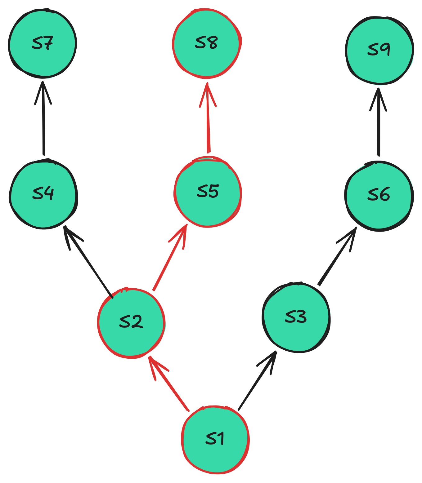
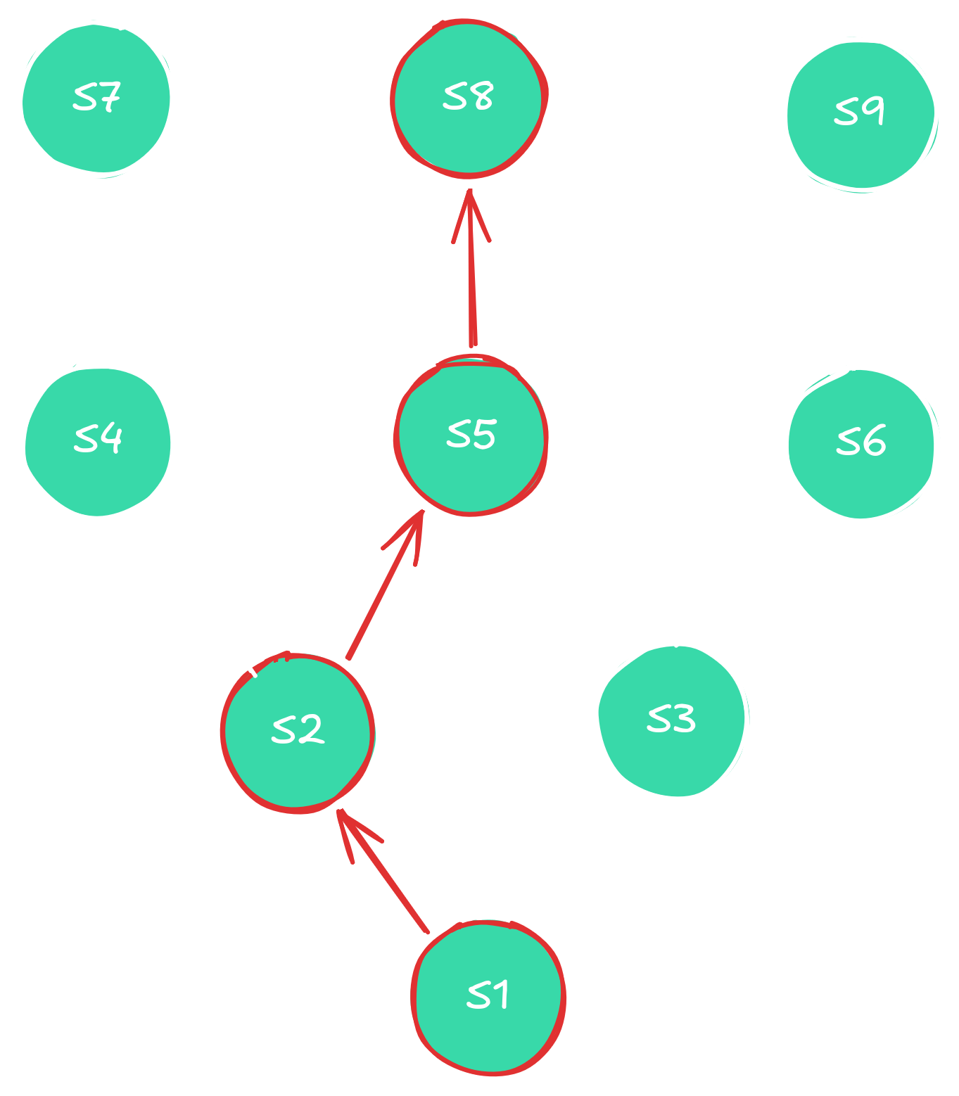
Mini example of a tree before creating the graph from it with an example trace of states to be parsed. We need to be sure that each of the nodes has seen enough
data samples so that its sampled distributions and predicted probabilities can be error bound for our purposes.
Mini example of a tree before creating the graph from it with an example trace of states to be parsed. We need to be sure that each of the nodes has seen enough
data samples so that its sampled distributions and predicted probabilities can be error bound for our purposes.
So now that we know we can bound the merge heuristic, and we can find the right states in the automaton, all that is missing is making sure that the transition probabilities are correct. Luckily, while differing in
our merge heuristic and employing a different streaming framework, we estimate the outgoing probabilities analogous to Palmer and Goldberg, and our proof so far has layer the groundwork to follow their analysis on
the transition probabilities one on one. Thus we did not elaborate on this part in our paper, but instead again refer to
their work. The basic idea however is once again making sure that each state sees enough samples, so that errors on probabilities can be bound.
For us in turn, all that is left is stitching it all together with the last theorem:
Theorem 10: Given a target PDFA $A$ and given our streaming strategy along with our merge heuristic. Given the required input parameters $L', n', \mu', \Sigma, \epsilon, \delta$, then for each
$L'\geq L$, $\mu' \leq \mu$, and $n' \geq n$ our framework returns a hypothesis automaton $H$ such that with probability at least $1-\delta$ the error is bounded by $L_1(H, A)\leq \epsilon$.
With this we can conclude that our learner indeed satisfies PAC-bounds, and throughout the analysis we showed what needs to be satisfied in order for the bounds to happen. However, our runtime of the algorithm
shows that our PAC-learner is not an efficient PAC-learner. The end of the paper section thus shows a modification of the algorithm that can be done
when the sample size per sketch is sufficiently large, greatly simplifying our algorithm and improving runtime. We did not test this modification experimentally, but we consider it a great theoretical improvement
that works on larger data sizes. We leave it up to the community to build on the idea.
On non-optimal solutions
Now this is all nice and well, but one can note that we don't have explicit guarantees, and therefore the whole concept is shaky at best. While I do acknowledge the limitations of the approach,
I briefly want to address the rightfully critical mind's concerns. The first thing I want to note is the following: Pretty much all of contemporary ML algorithms run on the same assumptions.
I do know that there is foundational work on the mathematical framework of deep learning (see e.g. works of this interesting scholar,
e.g. a publication on benign overfitting), but regardless of that, analyses normally focus on small models only so far.
In other words, these theoretical bounds do not hold for the extremely large models that have popped up over the past years. They might be discovered some day, but for now the common approach is
still to simply train and cushion against the worst cases through empirical testing.
A second argument can be made just by studying 'classical' algorithmic design. Specifically, we want to take a look at two examples of algorithms that are non-optimal, but still worth looking at.
The first one is an example of a randomized algorithm, i.e. it is non-deterministic. The algorithm is not the optimal algorithm for the problem it solves, but it serves as a good example
how random algorithms are still capable to find elegant solutions for difficult problems. The second algorithm we briefly touch on solves the infamous Knapsack problem, an instance of an
NP-hard problem.
Karger's algorithm for the min-cut problem
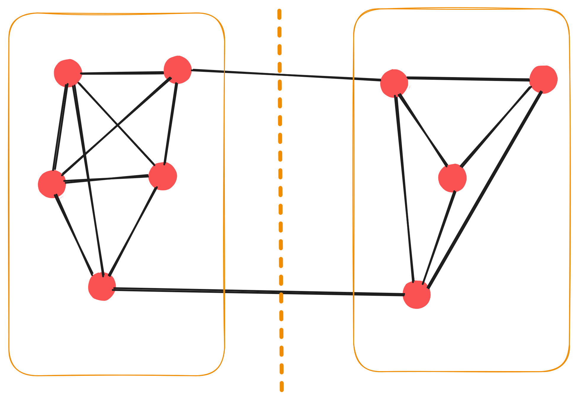
Karger's algorithm for the min-cut problem on graphs is a classical example in a good curriculum to show that simple algorithms can elegantly achieve desired results. The min-cut problem
essentially states as the following. Given a graph ($V$, $E$), find two partitions $G$, $H$, s.t. $G \cup H = V$ and that the set of edges crossing the two sets are minimal.
Example mini-graph with a minimum-cut solution. The min-cut separates the graph into two virtual components, connected through a minimum number of edges. Applications are e.g. finding vulnerabilities
in one's system, say a distributed system, to make it more robust against fallouts.
Example mini-graph with a minimum-cut solution. The min-cut separates the graph into two virtual components, connected through a minimum number of edges. Applications are e.g. finding vulnerabilities
in one's system, say a distributed system, to make it more robust against fallouts.
The algorithm itself is random and does not guarantee an optimial solution. Instead it gives you only a few lines of pseudocode to describe it fully:
Karger's random contraction algorithm
While there are more than two nodes/vertices do:
Pick a random edge $(u, v)\in E$ uniformly
Contract $u$ and $v$ into a single nodes/vertex
Remove self-loops from contracted node/vertext
It is clearly sleek and elegant in its pseudocode, and so is the mathematical analysis. Because we are not guaranteed to find the correct solution the algorithm is normally run multiple times, and
the solution which minimizes crossing edges is the correct solution. If we have $n$ nodes and do $N$ trials, then the probability of not finding the optimal solution (the true minimum), i.e. $P[all \text{ } trials \text{ } fail]$, is bounded
by $$P[all \text{ } trials \text{ } fail] \leq \left(1-\frac{1}{n^2}\right)^N.$$ Looking awfully familiar with $$\lim_{n \rightarrow \infty} \left(1-\frac{x}{n}\right)^n=e^x$$ we can perform e.g. $N=n^2$ trials, resulting in a
false solution bounded with probability $$P[all \text{ } trials \text{ } fail] \leq \frac{1}{e}.$$
Or alternatively we perform $N=n^2log(n)$ trials to get the even smoother bound $$P[all \text{ } trials \text{ } fail] \leq \frac{1}{n}.$$
The benefits of this algorithm are clearly its simplicity and elegant math, not its practicality, justifying its academic nature. There exist deterministic solutions solving the same problem in better
asymptotic time. However, sometimes we do not have this luxury and need to resort to randomized algorithms that do not always give the best solution, but give it only with a certain probability. This example was
to show that algorithms that do not always find the optimal solution do have a legitimate place in the overarching toolbox of algorithms. In fact, many algorithms inside of the very computers we use are not
optimal, but good enough. Optimal caching and the Bankers algorithm for instance both rely on knowlede of the future, clearly a real world contraint, which is why the clever engineers who designed our systems cooked up
approximate solutions or entirely different ones to solve these problems. The second example below may prove to be an even better example to illustrate trade-offs we have to make in algorithms sometimes.
Fully polynomial time approximation scheme for the Knapsack problem
The fully polynomial time approximation scheme (FPTAS) for the Knapsack problem is an algorithm to approximate the optimal solution. The exact algorithm yields
the solution in $O(nW)$ by means of dynamic programming, where $n$ is the number of items, and $W$ is the capacity of the bag, is NP-complete. That means we can't solve it in polynomial time (looking at the run-time that fact looks
very counterintuitive, worth thinking about). To solve the bottleneck an approximation algorithm exists. The basic idea of the algorithm is to find a value $v_{max}$ over all the items we get as input, then scale all weights by a factor
of $\frac{1}{m}$, rounding towards the floor. With that we can define a recurrence s.t. for an arbitrary value $\epsilon$ we can choose $m$ s.t.
$$m=\frac{\epsilon v_{max}}{n},$$
we get a solution $V_{approx}$ that is guaranteed to satisfy
$$V_{approx} \geq (1-\epsilon) V_{opt},$$
with $V_{opt}$ the optimal solution. The run-time of the approximation is $O(n^2 v_{max})$, a polynomial solution for small $v_{max}$. For more information on the algorithm I refer
to Wikipedia.
This example relates well to our algorithm. Both use a heuristic to simplify a computationally complex problem, and both give approximation guarantees. The difference is that the Knapsack problem
has an optimal solution that can be reached precily given some input, whereas the ground truth of the PDFA we are learning might or might not even be feasible, depending on what data points we
get to see. Hence we have to retreat to PAC-bounds territory.
In practice we could simply note that guarantees exist while simply running the algorithm and accepting that the solution might not be
the optimal solution. But it still might be good enough for our purposes. And this, i.e. the notion of what is good enough, is something we can control by understanding the algorithm and its limits,
and by setting our hyperparameters according to our needs.
Wrapping up
... and there went 2 months of my lifetime. However, I hope you got a little more familiar with some techniques and how to use them. Essentially PAC-bounds proofs need a series of
subsequent bounding, where each step provides the foundation for the next one, similar to system design almost. The bounds will reveal how to choose parameters such that the bounds
are fulfilled. In practice those numbers often get really large however, so often the bounds only serve a theoretical purpose, showing that at least in theory the algorithm has
guarantees.
As an upside to all this however we have mathematical guarantees that our learner does learn the correct result. If we wanted to we could bake those found parameters into the actual
algorithm and have it run on a real data stream, say a network of computers. Under the assumption that there is a natural behavior of the network (similar to say energy consumption
in an energy network: In the evening everbody goes home turns on the light, hence more activity in the evenings and less during daytime for private households), then a model for
the network can be built. And if we choose our parameters correctly we can be probably approximately sure (pun intended) that the result will be correct, and the model will be able
to raise alarms on anomalies.
More importantly: If you enjoyed this article or want to stay connected please feel free to reach out. You can find me on
LinkedIn and GitHub.